
Introduction to Probability and Statistical Distributions
Statistics forms the foundation of decision-making across industries, from healthcare to finance to engineering. At the heart of statistical analysis lies the concept of probability distributions, which describe how values of a random variable are spread across a range. Among all probability distributions, one stands out as particularly significant: the normal distribution. This mathematical model has become indispensable in countless fields because it accurately represents the behavior of real-world data in many situations.
The normal distribution, also known as the Gaussian distribution or bell curve, is a continuous probability distribution that exhibits remarkable properties and widespread applicability. Understanding this distribution is essential for anyone working with data, as it underpins many statistical methods and enables professionals to make informed predictions and decisions based on data analysis.
Defining the Normal Distribution: Core Characteristics
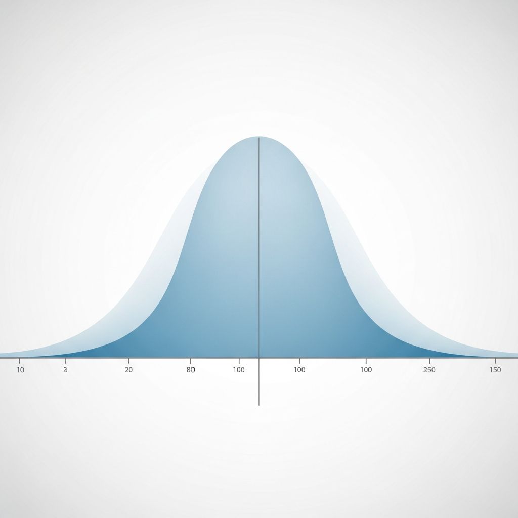
At its foundation, the normal distribution is a theoretical model that describes how values for a population are distributed. Rather than having values clustered randomly, a normal distribution follows a predictable, symmetrical pattern. The distribution gets its colloquial name “bell curve” from its distinctive shape when plotted on a graph.
The mathematical elegance of the normal distribution lies in its complete definition by just two parameters:
- Mean (μ): The central value around which data clusters, representing the average of all values
- Standard Deviation (σ): A measure of how spread out the data is from the mean
These two parameters fully determine the shape and position of the distribution. Any normal distribution can be expressed as X ~ N(μ, σ), indicating that variable X follows a normal distribution with mean μ and standard deviation σ.
Essential Properties of the Normal Distribution
The normal distribution possesses several defining characteristics that make it uniquely valuable for statistical analysis:
- Symmetry: The distribution is perfectly symmetrical around its mean, meaning the right side mirrors the left side exactly. This symmetry implies that extreme values above the mean are equally likely as extreme values below it.
- Bell Shape: When plotted graphically, the distribution forms a smooth, bell-shaped curve with the peak at the mean. The curve gradually tapers off as it extends toward extreme values.
- Mean-Median-Mode Equivalence: In a normal distribution, the mean, median, and mode are all identical, all occurring at the center of the distribution. This convergence of central tendency measures is unique to the normal distribution.
- Probability Area: The area under the entire curve always equals exactly 1, representing 100% of the probability. Any specific probability can be calculated by finding the area under the curve between two points.
- Central Concentration: Most data values cluster around the mean, with values becoming progressively less frequent as distance from the mean increases. This concentration means that typical values are far more likely than extreme values.
The Standard Normal Distribution: Foundation of Statistical Methods
While infinitely many normal distributions exist (each with different means and standard deviations), one particular normal distribution serves as a reference point for all others: the standard normal distribution. This special case occurs when the mean equals zero (μ = 0) and the standard deviation equals one (σ = 1).
The standard normal distribution, often denoted as Z, is described by the probability density function:
f(z) = (1/√(2π)) × e^(-z²/2)
This mathematical foundation allows statisticians to convert any normal distribution into the standard form through a process called standardization. By transforming values using the formula Z = (X – μ)/σ, researchers can use standardized tables and statistical tools to analyze any normal distribution.
The 68-95-99.7 Rule: Understanding Data Distribution
One of the most practical applications of normal distribution theory is the empirical rule, commonly known as the 68-95-99.7 rule. This guideline describes precisely how much of the data falls within specific distances from the mean, measured in standard deviations.
The empirical rule states the following percentages:
| Standard Deviations from Mean | Percentage of Data Within Range |
|---|---|
| 1 standard deviation (±1σ) | Approximately 68% |
| 2 standard deviations (±2σ) | Approximately 95% |
| 3 standard deviations (±3σ) | Approximately 99.7% |
This rule provides immediate insight into data concentration. For instance, in a distribution of adult heights, approximately 68% of people fall within one standard deviation of the mean height. Understanding this rule enables quick identification of unusual values: a height more than three standard deviations from the mean would be extraordinarily rare, appearing in less than 0.3% of the population.
Real-World Applications and Phenomena
The normal distribution’s prevalence in nature and human measurements makes it invaluable for practical applications. Many naturally occurring phenomena follow normal distributions, particularly when multiple independent factors influence the outcome:
- Physical Measurements: Heights, weights, and other body measurements in populations typically follow normal distributions, allowing scientists to characterize typical ranges and identify outliers.
- Test Scores and Academic Performance: Intelligence quotients (IQs), standardized test scores, and academic performance metrics frequently exhibit normal distribution patterns across populations.
- Biological Phenomena: Durations of pregnancies, lengths of biological cycles, and other physiological measurements often conform to normal distribution models.
- Manufacturing and Quality Control: Product dimensions, manufacturing tolerances, and quality metrics commonly follow normal distributions, enabling companies to establish acceptable ranges and detect defects.
- Financial Markets: Returns on investments and price changes, while not perfectly normal, often approximate normal distributions for analytical purposes in finance and risk management.
Why Normal Distribution Matters: Statistical Significance
The normal distribution’s importance in statistics extends far beyond merely describing data patterns. Due to the central limit theorem, the normal distribution becomes increasingly appropriate as a model even when underlying data sources are not perfectly normal. This property makes the normal distribution the foundation of many statistical inference methods, hypothesis testing approaches, and confidence interval calculations.
Additionally, the normal distribution possesses unique mathematical properties that no other continuous distribution shares. It is the only distribution whose cumulants beyond the first two (mean and variance) are zero, and it is the continuous distribution with maximum entropy for a specified mean and variance. These properties make it especially tractable for mathematical analysis and theoretical development.
Transforming Data: From Any Normal Distribution to Standard Form
The relationship between different normal distributions and the standard normal distribution enables powerful analytical flexibility. If Z represents a standard normal random variable, then the transformation X = σZ + μ produces a normal distribution with mean μ and standard deviation σ. This mathematical relationship means any normal distribution can be scaled and shifted from the standard form, or conversely, any normal distribution can be converted to standard form through the standardization transformation.
This capability allows analysts to use standardized statistical tables and software functions designed for the standard normal distribution to solve problems involving any normal distribution, dramatically simplifying calculations and analysis.
Recognizing Limitations and Departures from Normality
While the normal distribution provides an excellent model for many phenomena, real-world data does not always perfectly conform to this idealized distribution. Some datasets may be skewed, with values clustering more toward one end of the range. Others may have heavier tails than the normal distribution predicts, meaning extreme values occur more frequently than expected. Recognition of these departures from normality is important for selecting appropriate statistical methods and ensuring analytical accuracy.
Frequently Asked Questions
Q: Why is the normal distribution called “Gaussian”?
A: The normal distribution is named after Carl Friedrich Gauss, the influential mathematician who extensively studied this distribution and contributed significantly to its mathematical theory and applications in the early 19th century.
Q: Can a normal distribution have a negative mean?
A: Yes, the mean of a normal distribution can be any real number, including negative values. The mean simply determines where the center of the bell curve is positioned on the number line.
Q: What percentage of data falls outside three standard deviations?
A: According to the 68-95-99.7 rule, approximately 99.7% of data falls within three standard deviations of the mean, leaving approximately 0.3% in the extreme tails beyond three standard deviations.
Q: How does the standard deviation affect the shape of the normal distribution?
A: A larger standard deviation creates a wider, flatter bell curve with data more spread out, while a smaller standard deviation creates a narrower, taller curve with data clustered more tightly around the mean.
Q: Is human height a perfect normal distribution?
A: While human height approximately follows a normal distribution within populations, real data may show slight departures from perfect normality due to various biological and environmental factors affecting different groups.
Q: What is the relationship between the normal distribution and probability?
A: The area under the normal distribution curve between any two points represents the probability that a randomly selected value falls within that range, with the total area under the entire curve equaling 1 or 100%.
References
- Normal distribution — Monash University Student Academic Success. 2024. https://www.monash.edu/student-academic-success/mathematics/probability-and-distributions/normal-distribution
- Normal distribution — Wikipedia. 2025. https://en.wikipedia.org/wiki/Normal_distribution
- Normal Distribution | Introduction to Statistics — JMP Statistical Software by SAS. 2024. https://www.jmp.com/en/statistics-knowledge-portal/inferential-statistics/probability-distributions/normal-distribution
- The Normal Distribution — Utah State University Department of Mathematics. 2024. https://www.usu.edu/math/schneit/StatsStuff/Probability/probModels9
- Normal Distribution | Brilliant Math & Science Wiki — Brilliant Learning Platform. 2025. https://brilliant.org/wiki/normal-distribution/
- Bell Shaped Curve: Normal Distribution In Statistics — Simply Psychology. 2024. https://www.simplypsychology.org/normal-distribution.html

- Integrated M.A. in Applied Linguistics, University of Hyderabad
- 5+ years in editorial, instructional, SEO, and research-based writing
Sneha is a relationships and lifestyle writer with a strong foundation in applied linguistics and certified training in relationship coaching. She brings over five years of writing experience to theskillvault, crafting thoughtful, research-driven content that empowers readers to build healthier relationships, boost emotional well-being, and embrace holistic living. Her writing and insights reflect the belief that beauty, happiness, and wellness…