
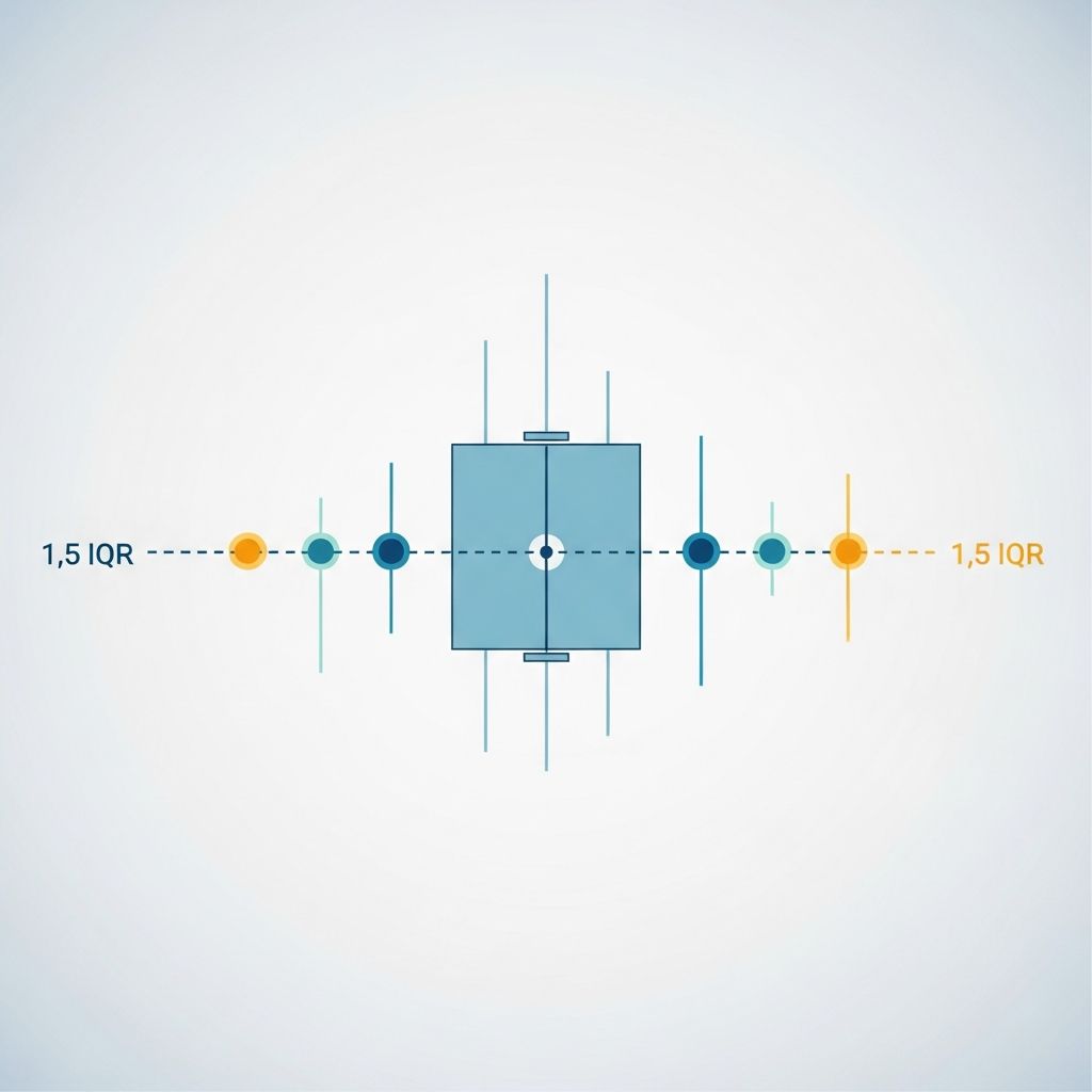
The **1.5 IQR rule** serves as a cornerstone in statistical analysis for pinpointing outliers—those data points that deviate significantly from the rest of the dataset. By leveraging the interquartile range (IQR), this method provides a reliable, distribution-agnostic approach to cleaning data and enhancing the accuracy of further analyses.
Understanding Quartiles and the Interquartile Range
Before diving into outlier detection, it’s essential to grasp the foundational concepts of quartiles. Quartiles divide an ordered dataset into four equal parts, each containing 25% of the data points.
- First Quartile (Q1): The value below which 25% of the data lies.
- Second Quartile (Q2): The median, where 50% of the data falls below.
- Third Quartile (Q3): The value below which 75% of the data lies.
The **interquartile range (IQR)** is calculated simply as IQR = Q3 – Q1. This metric captures the spread of the central 50% of the data, making it robust against extreme values that might skew other measures like the full range.
Why IQR Matters in Data Analysis
Unlike the total range (maximum minus minimum), which is highly sensitive to outliers, the IQR focuses on the middle portion of the data. This property gives it a high breakdown point of 25%, meaning it remains stable even if up to 25% of the data are outliers.
For instance, in a symmetric distribution, half the IQR approximates the median absolute deviation (MAD), another robust measure of variability.
Step-by-Step Guide to Calculating IQR
Computing the IQR involves sorting the data and finding the quartiles. Here’s a systematic process:
- Sort the dataset in ascending order.
- Locate the median (Q2): For an odd number of observations, it’s the middle value; for even, the average of the two central values.
- Find Q1: Median of the lower half (excluding Q2 if n is odd).
- Find Q3: Median of the upper half.
- Compute IQR: Subtract Q1 from Q3.
Example Calculation: Student Test Scores
Consider this dataset of 11 test scores: 65, 72, 78, 82, 85, 88, 90, 92, 95, 98, 105.
| Step | Calculation | Value |
|---|---|---|
| 1. Sorted Data | – | 65, 72, 78, 82, 85, 88, 90, 92, 95, 98, 105 |
| 2. Median (Q2) | 6th value | 88 |
| 3. Lower Half | 65, 72, 78, 82, 85 | Median Q1 = 78 |
| 4. Upper Half | 90, 92, 95, 98, 105 | Median Q3 = 95 |
| 5. IQR | Q3 – Q1 | 95 – 78 = 17 |
This IQR of 17 indicates moderate variability in the central scores.
The 1.5 IQR Rule Explained
The 1.5 IQR rule defines outliers as data points falling outside the fences: Lower Fence = Q1 – 1.5 × IQR and Upper Fence = Q3 + 1.5 × IQR. Values below the lower fence or above the upper fence are flagged as outliers.
This multiplier of 1.5 is chosen because it aligns closely with the Gaussian distribution, where Q1 and Q3 are approximately ±0.675 standard deviations from the mean. Thus, 1.5 IQR covers about 99.3% of the data in normal distributions, leaving extremes as outliers.
Visualizing the Fences
Imagine a box plot: the box spans Q1 to Q3, with whiskers extending to the fences. Points beyond are plotted separately as outliers.
- Mild Outliers: Beyond 1.5 IQR (standard rule).
- Extreme Outliers: Sometimes defined at 3 IQR for even stricter criteria.
Applying the Rule: Real-World Example
Using the previous scores: Q1=78, Q3=95, IQR=17.
- 1.5 × IQR = 1.5 × 17 = 25.5
- Lower Fence: 78 – 25.5 = 52.5
- Upper Fence: 95 + 25.5 = 120.5
Here, 105 is within 120.5, so no outliers. But if we add a score of 140:
- 140 > 120.5 → Outlier detected!
This flags unusually high performances, possibly due to errors or extraordinary circumstances.
Advantages of the 1.5 IQR Method
This approach excels in several ways:
- Non-parametric: No assumption of normality required.
- Robust: Unaffected by extreme values in calculation.
- Visual-Friendly: Integrates seamlessly with box plots.
- Consistent: Standard across statistical software like R, Python (pandas), and Excel.
Limitations and Considerations
While powerful, the method isn’t flawless:
- May flag legitimate points in skewed distributions.
- Small datasets (<10 points) can produce unreliable quartiles.
- Doesn’t explain why a point is an outlier—further investigation needed.
For multimodal data, consider domain knowledge or alternative methods like z-scores.
Outlier Detection in Software
Python Example with Pandas
import pandas as pdimport numpy as npdata = [65, 72, 78, 82, 85, 88, 90, 92, 95, 98, 105, 140]df = pd.DataFrame(data, columns=['scores'])Q1 = df['scores'].quantile(0.25)Q3 = df['scores'].quantile(0.75)IQR = Q3 - Q1lower_fence = Q1 - 1.5 * IQRupper_fence = Q3 + 1.5 * IQRoutliers = df[(df['scores'] < lower_fence) | (df['scores'] > upper_fence)]print("Outliers:", outliers)This code outputs 140 as an outlier.
R Code Snippet
data <- c(65, 72, 78, 82, 85, 88, 90, 92, 95, 98, 105, 140)Q1 <- quantile(data, 0.25)Q3 <- quantile(data, 0.75)IQR <- IQR(data)outliers <- data[data < (Q1 - 1.5*IQR) | data > (Q3 + 1.5*IQR)]print(outliers)Advanced Applications and Variations
Beyond basics, the IQR rule adapts to various fields:
- Finance: Detecting anomalous transactions.
- Healthcare: Identifying unusual patient vitals.
- Machine Learning: Preprocessing for robust models.
Variations include adjusting the multiplier (e.g., 3 for extreme outliers) or using modified Z-scores based on MAD.
Common Misconceptions Debunked
| Myth | Fact |
|---|---|
| IQR assumes normal distribution | False—it’s non-parametric. |
| All outliers should be removed | No—investigate first; they may be valid. |
| 1.5 is arbitrary | Derived from Gaussian properties. |
Frequently Asked Questions (FAQs)
What if my dataset has an even number of points?
Average the two middle values for the median, then split halves accordingly for Q1 and Q3.
Can I use IQR for categorical data?
No—IQR applies to numerical, ordered data only.
How does IQR compare to standard deviation?
IQR is more robust to outliers; SD is sensitive.
Is 1.5 IQR the only multiplier?
Common standard, but 2.0 or 3.0 used for different sensitivities.
What about ties in data?
Quartile methods handle ties via interpolation; software automates this.
Practical Tips for Implementation
To maximize effectiveness:
- Always plot data (box plots) alongside calculations.
- Combine with domain expertise for validation.
- For large datasets, use bootstrapping for quartile stability.
- Document decisions on outlier handling.
In summary, the 1.5 IQR rule empowers analysts to make data-driven decisions with confidence, balancing sensitivity and robustness in outlier detection.
References
- Interquartile range – Wikipedia — Wikipedia contributors. 2023-10-15. https://en.wikipedia.org/wiki/Interquartile_range
- Determining an Outlier Using the 1.5 IQR Rule — YouTube (Real World Statistics). 2015-01-01. https://www.youtube.com/watch?v=rZJbj2I-_Ek
- 3.2 – Identifying Outliers: IQR Method — Penn State University (STAT 200). 2023-01-01. https://online.stat.psu.edu/stat200/lesson/3/3.2
- 1.5 IQR Rule Explained — Built In. 2023-05-10. https://builtin.com/articles/1-5-iqr-rule
- The Interquartile Range Method For Outliers — ProCogia. 2023-08-20. https://procogia.com/interquartile-range-method-for-reliable-data-analysis/
- Identifying outliers with the 1.5xIQR rule — Khan Academy. 2023-01-01. https://www.khanacademy.org/math/statistics-probability/summarizing-quantitative-data/box-whisker-plots/a/identifying-outliers-iqr-rule
- Interquartile Range to Detect Outliers in Data — GeeksforGeeks. 2024-02-15. https://www.geeksforgeeks.org/machine-learning/interquartile-range-to-detect-outliers-in-data/

- Integrated M.A. in Applied Linguistics, University of Hyderabad
- 5+ years in editorial, instructional, SEO, and research-based writing
Sneha is a relationships and lifestyle writer with a strong foundation in applied linguistics and certified training in relationship coaching. She brings over five years of writing experience to theskillvault, crafting thoughtful, research-driven content that empowers readers to build healthier relationships, boost emotional well-being, and embrace holistic living. Her writing and insights reflect the belief that beauty, happiness, and wellness…