Linear Equations: Methods for Solving Systems and Single Equations

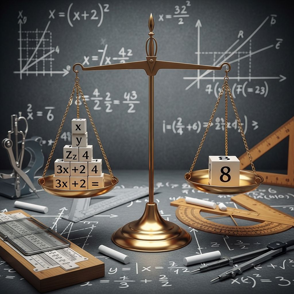
Understanding the Foundation of Linear Equations

Linear equations form the backbone of algebra and serve as a gateway to understanding more complex mathematical concepts. A linear equation is a mathematical statement that contains variables and constants combined through addition, subtraction, multiplication, or division, with the highest power of the variable being one. These equations appear in numerous real-world applications, from calculating costs and distances to predicting trends and analyzing relationships between quantities.

The primary objective when working with linear equations is to determine the value of the unknown variable that makes the equation true. This process, known as solving, requires applying systematic methods that transform the equation into simpler forms until the variable stands isolated on one side of the equation. Understanding these foundational principles enables students to approach increasingly difficult problems with confidence and precision.

Core Principles for Equation Manipulation

Before diving into specific solving techniques, it is essential to grasp the fundamental principles that govern equation manipulation. The properties of equality form the theoretical foundation for all algebraic operations. When any operation is performed on one side of an equation, the same operation must be applied to the other side to maintain balance. This principle ensures that the two sides of the equation remain equivalent throughout the solving process.

The key properties include:

• Addition Property: Adding the same number to both sides preserves equality
• Subtraction Property: Subtracting identical values from both sides maintains the equation’s validity
• Multiplication Property: Multiplying both sides by the same non-zero number keeps the equation balanced
• Division Property: Dividing both sides by the same non-zero number preserves equality

These properties allow mathematicians to transform equations systematically while maintaining their essential truth. By applying these operations strategically, any linear equation can be solved through a series of logical steps.

The Substitution Technique for System Solutions

The substitution method provides an elegant approach for solving systems of linear equations involving two or more variables. This technique involves identifying one equation where a variable can be easily isolated, then replacing that variable in the second equation with its equivalent expression. The result is a single equation containing only one unknown quantity, which can be solved using standard algebraic operations.

The substitution approach follows a structured sequence:

1. Select one of the given equations and rearrange it to express one variable in terms of the other variables and constants
2. Substitute this expression into the remaining equation, replacing all instances of the isolated variable
3. Solve the resulting single-variable equation using basic algebraic techniques
4. Once the first variable’s value is determined, substitute it back into one of the original equations to find the remaining variable’s value
5. Verify the solution by substituting both values into both original equations

This method proves particularly effective when one of the equations naturally expresses a variable with a coefficient of one, making isolation straightforward and minimizing computational complexity.

The Elimination Method for Systematic Reduction

The elimination method, also called the addition-subtraction method, takes a different approach by strategically combining equations to cancel out variables. Rather than substituting expressions, this technique multiplies one or both equations by carefully chosen constants, creating equal coefficients for one variable across equations. When these modified equations are added or subtracted, one variable vanishes, leaving a single-variable equation to solve.

The elimination method process unfolds as follows:

1. Examine both equations to identify which variable would be most convenient to eliminate based on existing coefficients
2. Multiply one or both equations by appropriate constants so that one variable has identical coefficients in both equations (though possibly with opposite signs)
3. Add or subtract the resulting equations to eliminate the targeted variable
4. Solve the single-variable equation that results from the elimination
5. Substitute the calculated value back into either original equation to find the other variable
6. Check the solution against both original equations

The elimination method shines when coefficients are already similar or when creating equal coefficients through multiplication results in manageable numbers. It often produces cleaner calculations compared to other methods, particularly when dealing with fractions or decimals in the original equations.

Cross Multiplication for Specialized Equation Forms

The cross multiplication method applies specifically to equations containing ratios or fractions. This technique utilizes the fundamental property that if two fractions are equal, then the product of the numerator of the first fraction and the denominator of the second fraction equals the product of the numerator of the second fraction and the denominator of the first fraction. Cross multiplication efficiently eliminates fractional components in a single step, simplifying subsequent calculations.

When encountering an equation of the form (a/b) = (c/d), cross multiplication yields ad = bc. This transformation removes fractions entirely and creates a linear equation that standard algebraic techniques can readily solve. The method proves invaluable when dealing with proportions, rates, or equations naturally expressed in fractional form.

Graphical Representation and Visual Solutions

While algebraic methods provide precise numerical answers, graphical techniques offer valuable visual insight into equation behavior. Each linear equation can be represented as a line on a coordinate plane. For a system of two linear equations with two variables, plotting both lines reveals their solution at the point of intersection. The x-coordinate and y-coordinate of this intersection point directly represent the values of the variables that satisfy both equations simultaneously.

The graphical method involves:

• Rearranging each equation into slope-intercept form (y = mx + b)
• Identifying the y-intercept and slope for each equation
• Plotting both lines accurately on a coordinate grid
• Locating the point where the lines cross
• Reading the coordinates of the intersection point as the solution

The graphical approach provides intuitive understanding of why systems have unique solutions, infinitely many solutions (when lines coincide), or no solutions (when lines run parallel). This visualization reinforces the algebraic principles underlying equation solving.

Step-by-Step Example: Applying the Substitution Approach

Consider the system: 3x + y = 13 and 2x + 3y = 18. Using substitution, the first equation can be rearranged to express y in terms of x: y = 13 – 3x. This expression is then substituted into the second equation, yielding 2x + 3(13 – 3x) = 18. Expanding and simplifying: 2x + 39 – 9x = 18, which reduces to -7x + 39 = 18. Subtracting 39 from both sides gives -7x = -21, and dividing by -7 produces x = 3. Substituting x = 3 back into y = 13 – 3x yields y = 13 – 9 = 4. The solution (3, 4) can be verified in both original equations.

Step-by-Step Example: Implementing the Elimination Approach

Using the same system (3x + y = 13 and 2x + 3y = 18), the elimination method multiplies the first equation by 3: 9x + 3y = 39. Subtracting the second equation (2x + 3y = 18) from this result eliminates y: 7x = 21, so x = 3. Substituting x = 3 into the first equation: 9 + y = 13, therefore y = 4. This demonstrates how different methods arrive at identical solutions through different procedural paths.

Handling Complex Structures and Special Cases

Linear equations often contain complicating features such as parentheses, decimals, or variables appearing on both sides of the equation. Parentheses require applying the distributive property before beginning the standard solving sequence. Equations with decimals become simpler when both sides are multiplied by an appropriate power of ten, converting decimals to whole numbers. When variables appear on both sides, collecting all variable terms on one side and constants on the other creates a standard form equation.

Certain systems yield special solutions: when solving produces a true statement like 0 = 0, the system has infinitely many solutions (the equations represent the same line). Conversely, when the solving process generates a false statement like 0 = 5, the system has no solution (the equations represent parallel lines). Recognizing these special cases prevents confusion and correctly interprets the geometric meaning of the algebraic results.

Practical Problem-Solving Strategies

Selecting the optimal solving method depends on the equation’s structure and coefficients. If one variable already has a coefficient of one or negative one, substitution typically minimizes computational steps. If coefficients are already similar or multiply to convenient values, elimination often proves faster. When equations naturally contain fractions, cross multiplication frequently offers the most direct path. Developing the judgment to match method to problem characteristics improves both speed and accuracy.

Before beginning any solution process, simplifying both sides of the equation by combining like terms and applying the distributive property streamlines subsequent steps. Checking solutions by substituting calculated values into all original equations catches algebraic errors and builds confidence in results. Organizing work clearly with explicit steps aids understanding and makes errors easier to identify and correct.

Common Questions About Equation Solving

Q: Why must the same operation be applied to both sides of an equation?

A: Applying different operations to each side breaks the equality relationship. The equation represents a balance, and maintaining that balance requires performing identical operations to both sides.

Q: How do I know which solving method to use?

A: Examine the equation structure. Substitution works well when one variable is easily isolated. Elimination suits equations where coefficients are similar. Cross multiplication handles fractional equations efficiently. Graphical methods provide visual understanding.

Q: What does it mean when solving produces a false statement?

A: A false statement (like 0 = 5) indicates the system has no solution. This occurs when equations represent parallel lines that never intersect.

Q: Can fractional coefficients be avoided?

A: Yes, multiplying all terms by the least common multiple of denominators converts fractional coefficients to whole numbers, simplifying calculations substantially.

Q: Why verify solutions?

A: Verification confirms that calculated values satisfy the original equations, catching algebraic mistakes and validating the solving process.

Conclusion and Mastery Development

Solving linear equations represents a fundamental algebraic skill applicable across mathematics, science, engineering, and numerous practical fields. Multiple solution methods exist because different equation structures naturally lend themselves to different approaches. Substitution, elimination, cross multiplication, and graphical techniques each provide pathways to correct solutions. Proficiency develops through consistent practice with varied problems, allowing solvers to recognize patterns and select efficient strategies. By understanding the underlying principles governing equation manipulation and practicing diverse problem types, students build confidence and competence in this essential mathematical domain.

Written by

Sneha Tete

• Integrated M.A. in Applied Linguistics, University of Hyderabad
• 5+ years in editorial, instructional, SEO, and research-based writing

Sneha is a relationships and lifestyle writer with a strong foundation in applied linguistics and certified training in relationship coaching. She brings over five years of writing experience to theskillvault,  crafting thoughtful, research-driven content that empowers readers to build healthier relationships, boost emotional well-being, and embrace holistic living. Her writing and insights reflect the belief that beauty, happiness, and wellness…

References

- Solving Linear Equations — Cuemath. 2025. https://www.cuemath.com/algebra/solving-linear-equations/
- Solving Linear Equations- Part II — Mathematics LibreTexts, OpenStax. 2025. https://math.libretexts.org/Bookshelves/Algebra/Elementary_Algebra_(LibreTexts)/02:_Linear_Equations_and_Inequalities/2.04:_Solving_Linear_Equations-_Part_II
- Solving Linear Equations — Saylor Foundation. 2012. https://saylordotorg.github.io/text_intermediate-algebra/s04-07-solving-linear-equations.html
- Linear Equations – Math Steps, Examples & Questions — Third Space Learning. 2025. https://thirdspacelearning.com/us/math-resources/topic-guides/algebra/linear-equations/
- Solving systems of linear equations — Khan Academy. 2025. https://www.khanacademy.org/test-prep/v2-sat-math/x0fcc98a58ba3bea7:algebra-easier/x0fcc98a58ba3bea7:solving-systems-of-linear-equations-easier/a/v2-sat-lesson-solving-systems-of-linear-equations