
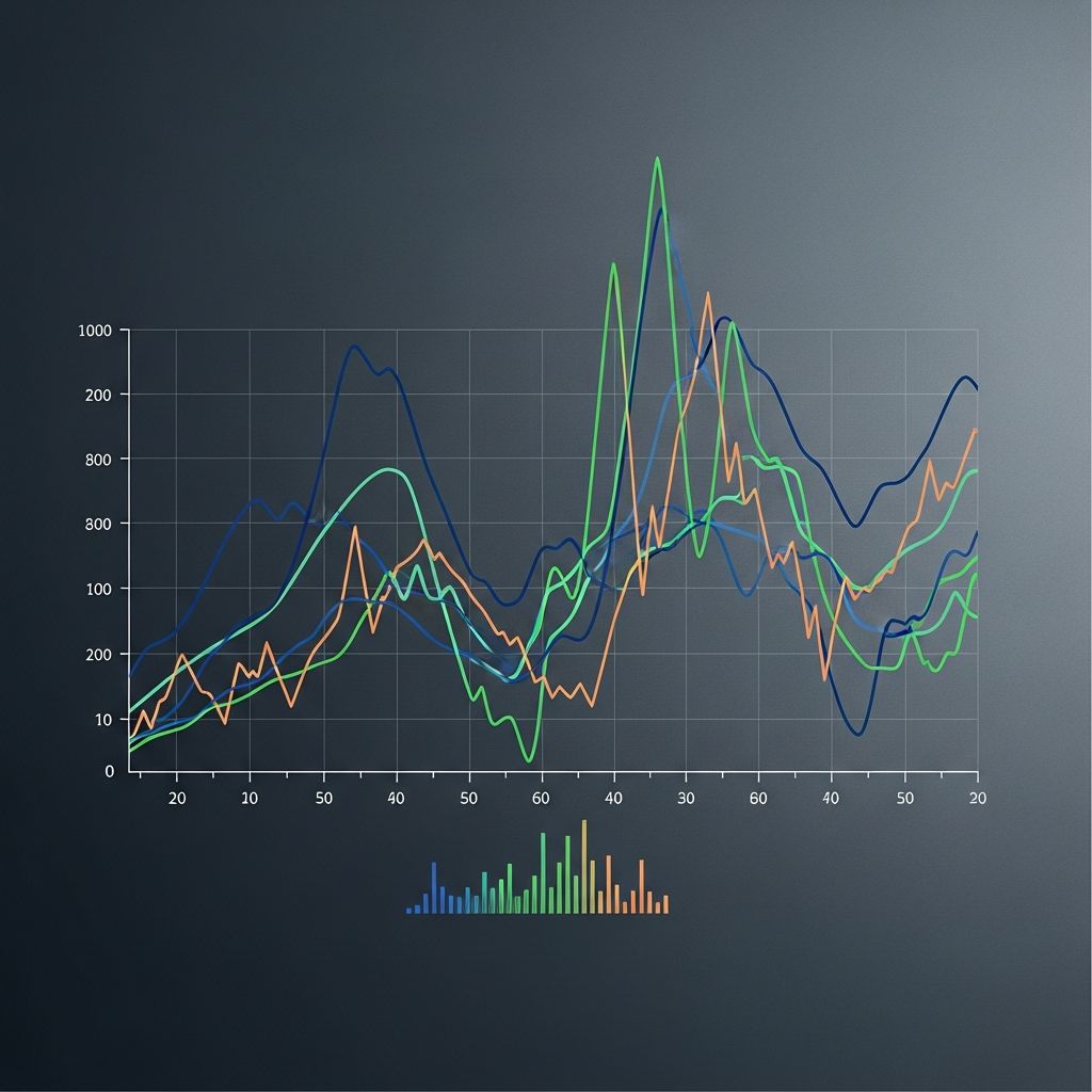
Time series graphs serve as powerful tools for representing sequential data points collected across regular intervals, enabling clear visualization of changes, developments, and projections over time. These visualizations plot temporal data on a line chart where the horizontal axis denotes time progression and the vertical axis captures the measured values, facilitating the detection of underlying patterns that inform decision-making in diverse sectors.
Defining Time Series Data and Graphs
At its core, a time series consists of observations recorded in chronological sequence, often at fixed intervals such as daily, monthly, or yearly marks. Unlike static charts that compare categories, time series graphs emphasize evolution, making them indispensable for tracking metrics like stock prices, temperatures, or sales figures. The mathematical foundation lies in discrete-time data points, each associated with a specific timestamp, allowing analysts to model temporal dependencies effectively.
These graphs transform raw numerical sequences into intuitive visuals by connecting plotted points with lines, revealing the narrative hidden in tables. For instance, economists use them to monitor GDP fluctuations, while meteorologists plot rainfall to predict seasonal variations. Their strength derives from preserving the natural order of events, which is crucial for accurate interpretation.
Core Components of a Time Series Graph
Every time series graph features two primary axes: the x-axis dedicated exclusively to time units—from seconds to decades—and the y-axis for the variable’s magnitude. Data points are positioned at intersections corresponding to their exact timestamps and values, then linked to form a continuous line that highlights continuity or abrupt shifts.
- Time Axis (X-Axis): Must progress left to right, using scales like hours, days, or years based on data granularity.
- Value Axis (Y-Axis): Scales according to the data range, often logarithmic for exponential growth.
- Data Points and Lines: Markers indicate individual observations; lines illustrate trajectories.
- Gridlines and Labels: Enhance readability by providing reference scales and clear annotations.
Additional elements like multiple lines for comparative series or shaded confidence intervals add depth, supporting multi-variable analysis without cluttering the view.
Step-by-Step Guide to Creating Time Series Graphs
Constructing a time series graph begins with data preparation: ensure timestamps are sequential and values are numeric. Aggregate if needed—summing daily sales into monthly totals—for smoother visuals.
- Select Software/Tools: Options range from Excel for basics to Python’s Matplotlib or R’s ggplot2 for advanced plotting.
- Define Axes: Assign time to x-axis, values to y-axis; choose appropriate intervals (e.g., weekly bins for hourly data).
- Plot Points: Input data to generate markers at precise coordinates.
- Connect and Customize: Draw lines, add titles like ‘Monthly Revenue 2020-2025’, legends, and color-coding.
- Validate: Check for distortions like uneven scaling that could mislead trends.
This process, detailed in analytical toolkits like ArcGIS Insights, ensures graphs align with data intervals from minutes to decades.
Identifying Key Patterns in Time Series Graphs
Time series graphs excel at unveiling four primary patterns: trends, seasonality, cycles, and irregularities.
| Pattern Type | Description | Example |
|---|---|---|
| Trend | Long-term increase or decrease | Rising global temperatures over decades |
| Seasonality | Repeating short-term cycles | Quarterly retail sales peaks during holidays |
| Cycle | Longer, irregular waves | Business boom-bust periods |
| Irregularity | Random noise or outliers | Sudden stock drop from news event |
Trends appear as steady slopes, seasonality as periodic waves, cycles as broader undulations, and irregularities as spikes. Recognizing these aids in decomposition—separating components for precise forecasting.
Real-World Applications Across Industries
In finance, time series graphs track stock indices like the Dow Jones, spotting bull markets or crashes via line trajectories. Meteorology relies on them for temperature or precipitation plots, essential for weather forecasting models. Businesses analyze website traffic or revenue streams to optimize strategies, while public health visualizes infection rates during pandemics to guide interventions.
Engineers monitor sensor data in real-time for predictive maintenance, and astronomers chart celestial events over centuries. These applications underscore the graph’s versatility in handling everything from high-frequency trading data to long-term climate records.
Advanced Variations and Techniques
Beyond basic lines, variations enhance complexity:
- Multi-Line Graphs: Overlay several series, like comparing product sales.
- Dual-Axis Charts: Accommodate disparate scales, e.g., revenue (left) vs. units sold (right).
- Area Plots: Fill under lines for cumulative effects, ideal for stacked metrics.
- Box Plots Over Time: Show distributions per interval for volatility insights.
Techniques like smoothing (moving averages) reduce noise, while decomposition isolates components mathematically. Forecasting extends patterns using models like ARIMA, visualized as extrapolated lines.
Common Pitfalls and Best Practices
Missteps can distort insights: starting x-axis at non-zero misrepresents changes; ignoring gaps fabricates continuity. Best practices include consistent scales, clear legends, and annotations for anomalies. Always contextualize with domain knowledge— a flat line might signal stability or stagnation.
For digital tools, ensure responsiveness for interactive exploration, zooming into peaks. Validate against raw data to confirm accuracy.
Frequently Asked Questions (FAQs)
What distinguishes a time series graph from a standard line graph?
A time series graph mandates time on the x-axis with data in chronological order, focusing on temporal evolution, whereas standard line graphs can plot any variables.
Can time series graphs handle missing data?
Yes, via interpolation or gap indicators, but transparency prevents false continuity assumptions.
Are they suitable for categorical data?
No, they require numerical values; convert categories to counts or frequencies first.
How do they support forecasting?
By extrapolating identified trends and seasonality, often paired with statistical models for predictions.
What software is best for beginners?
Excel or Google Sheets offer simple entry points; advance to Tableau or Python for sophistication.
Conclusion: Harnessing Time Series for Insights
Time series graphs distill complex temporal data into actionable visuals, empowering predictions and strategies across fields. Mastering their creation and interpretation unlocks deeper data understanding.
References
- What Is a Time Series Graph and How Does It Work — FanRuan. 2023-05-15. https://www.fanruan.com/en/blog/what-is-a-time-series-graph
- Time-Series Graphs: Types, Examples & How to Read — TigerData. 2024-02-20. https://www.tigerdata.com/blog/what-is-a-time-series-graph-with-examples
- Timeplot / Time Series: Definition, Examples & Analysis — Statistics How To. 2023-11-10. https://www.statisticshowto.com/timeplot/
- Time Series Plot — InfluxData. 2024-01-08. https://www.influxdata.com/glossary/time-series-plot/
- Time Series Graph – Math Steps, Examples & Questions — Third Space Learning. 2023-09-22. https://thirdspacelearning.com/us/math-resources/topic-guides/statistics-and-probability/time-series-graph/
- Create and use a time series graph — Esri ArcGIS Documentation. 2025-03-01. https://doc.arcgis.com/en/insights/latest/create/time-series.htm

Medha Deb is an editor with a master's degree in Applied Linguistics from the University of Hyderabad. She believes that her qualification has helped her develop a deep understanding of language and its application in various contexts. Medha specializes in the areas of beauty, health, sports, and wellness and is committed to ensuring that the content on the website is…